
Exploratory data analysis in R
You have some data to play with! Now what? The first step in any data project is to explore the data: what is the structure of your data? What variables do you have? What patterns jump out at you? This mini-tutorial covers the basics of exploratory data analysis in R.
Intro - why EDA?
- explore the data, could lead to new hypotheses
- looking for patterns (variation in data, covariation in data – from https://r4ds.had.co.nz/exploratory-data-analysis.html)
- distribution, skew, outliers
Parts of EDA
As Hadley Wickham wrote in his R for data science book, the main goal of EDA is looking at variation and covariation in data. In other words, what patterns do we see and how do the patterns of different variables relate?
The first step is to understand the structure of the data. Once we understand the structure of our data we can look at patterns in individual variables and finally look for covariation among variables.
- Data structure:
- variable type
- summarize variables
- Patterns:
- visualize summaries
- histograms
- Covariance:
- correlations
- boxplots
- scatter plots
- dimension reduction (PCA, NLDR)
Get some data!
To see these ideas in practice let’s load a dataset to play with. Here
we will use 2016 election poll data compiled by Rafael
Irizarry
in the dslabs package.
Start by installing the dslab package by running
install.packages("dslabs"). In this tutorial we will use and explore a
number of additional packages. To make sure that they are installed run:
install.packages(c("dplyr","skimr","SmartEDA","GGally","Hmisc","psych","summarytools","corrplot")).
If GGally package does not load try install_github("ggobi/ggally").
library(dslabs)
library(dplyr)
library(ggplot2)

polls <- polls_us_election_2016
1. Data Structure
dim(polls)
## [1] 4208 15
dim gives the dimensions of the data or the number of rows x number of
columns. Here we have 4208 x 15 which means 4208 rows of entries by 15
columns of variables.
glimpse(polls)
## Rows: 4,208
## Columns: 15
## $ state            <fct> U.S., U.S., U.S., U.S., U.S., U.S., U.S., U.S., Ne...
## $ startdate        <date> 2016-11-03, 2016-11-01, 2016-11-02, 2016-11-04, 2...
## $ enddate          <date> 2016-11-06, 2016-11-07, 2016-11-06, 2016-11-07, 2...
## $ pollster         <fct> ABC News/Washington Post, Google Consumer Surveys,...
## $ grade            <fct> A+, B, A-, B, B-, A, A-, A-, NA, A-, A+, A-, A+, B...
## $ samplesize       <int> 2220, 26574, 2195, 3677, 16639, 1295, 1426, 1282, ...
## $ population       <chr> "lv", "lv", "lv", "lv", "rv", "lv", "lv", "lv", "l...
## $ rawpoll_clinton  <dbl> 47.00, 38.03, 42.00, 45.00, 47.00, 48.00, 45.00, 4...
## $ rawpoll_trump    <dbl> 43.00, 35.69, 39.00, 41.00, 43.00, 44.00, 41.00, 4...
## $ rawpoll_johnson  <dbl> 4.00, 5.46, 6.00, 5.00, 3.00, 3.00, 5.00, 6.00, 6....
## $ rawpoll_mcmullin <dbl> NA, NA, NA, NA, NA, NA, NA, NA, NA, NA, NA, NA, NA...
## $ adjpoll_clinton  <dbl> 45.20163, 43.34557, 42.02638, 45.65676, 46.84089, ...
## $ adjpoll_trump    <dbl> 41.72430, 41.21439, 38.81620, 40.92004, 42.33184, ...
## $ adjpoll_johnson  <dbl> 4.626221, 5.175792, 6.844734, 6.069454, 3.726098, ...
## $ adjpoll_mcmullin <dbl> NA, NA, NA, NA, NA, NA, NA, NA, NA, NA, NA, NA, NA...
glimpse summarizes a number of characteristics of the data giving the
number of rows and columns, names of the variables, variable types, and
the first few rows of each column. The variable type is helpful to
understand how the data was entered. For instance, here state is entered
as a factor. But it could have been a character type. And knowing which
of those we are working with helps us understand how the data might
behave. Similarly, startdate is entered as a date type but it could
have been a character or factor. Seeing the first few rows of each
variable gives us an idea of the type of entries we expect to see.
glimpse is from the dplyr package.
head(polls)
##   state  startdate    enddate
## 1  U.S. 2016-11-03 2016-11-06
## 2  U.S. 2016-11-01 2016-11-07
## 3  U.S. 2016-11-02 2016-11-06
## 4  U.S. 2016-11-04 2016-11-07
## 5  U.S. 2016-11-03 2016-11-06
## 6  U.S. 2016-11-03 2016-11-06
##                                                     pollster grade samplesize
## 1                                   ABC News/Washington Post    A+       2220
## 2                                    Google Consumer Surveys     B      26574
## 3                                                      Ipsos    A-       2195
## 4                                                     YouGov     B       3677
## 5                                           Gravis Marketing    B-      16639
## 6 Fox News/Anderson Robbins Research/Shaw & Company Research     A       1295
##   population rawpoll_clinton rawpoll_trump rawpoll_johnson rawpoll_mcmullin
## 1         lv           47.00         43.00            4.00               NA
## 2         lv           38.03         35.69            5.46               NA
## 3         lv           42.00         39.00            6.00               NA
## 4         lv           45.00         41.00            5.00               NA
## 5         rv           47.00         43.00            3.00               NA
## 6         lv           48.00         44.00            3.00               NA
##   adjpoll_clinton adjpoll_trump adjpoll_johnson adjpoll_mcmullin
## 1        45.20163      41.72430        4.626221               NA
## 2        43.34557      41.21439        5.175792               NA
## 3        42.02638      38.81620        6.844734               NA
## 4        45.65676      40.92004        6.069454               NA
## 5        46.84089      42.33184        3.726098               NA
## 6        49.02208      43.95631        3.057876               NA
head shows us the first 6 rows of each column. This is helpful for
understanding the variable names, how the data is entered, and example
entries.
Sometimes we want to know what the unique values are for a variable. For
instance, let’s look at which pollsters were included in this dataset.
unique(polls$population)
## [1] "lv" "rv" "a" "v"
There were 4 population types: lv, rv, a, and v.
For numeric variables we want summary statistics. These can be computed
using the summary command which shows the minimum, 1st qartile, mean,
median, 3rd quartile, and maximum for each numeric variable.
summary(polls)
##             state        startdate             enddate
##  U.S.          :1106   Min.   :2015-11-06   Min.   :2015-11-08
##  Florida       : 148   1st Qu.:2016-08-10   1st Qu.:2016-08-21
##  North Carolina: 125   Median :2016-09-23   Median :2016-09-30
##  Pennsylvania  : 125   Mean   :2016-08-31   Mean   :2016-09-06
##  Ohio          : 115   3rd Qu.:2016-10-20   3rd Qu.:2016-10-28
##  New Hampshire : 112   Max.   :2016-11-06   Max.   :2016-11-07
##  (Other)       :2477
##                                      pollster        grade
##  Ipsos                                   : 919   A-     :1085
##  Google Consumer Surveys                 : 743   B      :1011
##  SurveyMonkey                            : 660   C-     : 693
##  YouGov                                  : 130   C+     : 329
##  Rasmussen Reports/Pulse Opinion Research: 125   B+     : 204
##  USC Dornsife/LA Times                   : 121   (Other): 457
##  (Other)                                 :1510   NA's   : 429
##    samplesize       population        rawpoll_clinton rawpoll_trump
##  Min.   :   35.0   Length:4208        Min.   :11.04   Min.   : 4.00
##  1st Qu.:  447.5   Class :character   1st Qu.:38.00   1st Qu.:35.00
##  Median :  772.0   Mode  :character   Median :43.00   Median :40.00
##  Mean   : 1148.2                      Mean   :41.99   Mean   :39.83
##  3rd Qu.: 1236.5                      3rd Qu.:46.20   3rd Qu.:45.00
##  Max.   :84292.0                      Max.   :88.00   Max.   :68.00
##  NA's   :1
##  rawpoll_johnson  rawpoll_mcmullin adjpoll_clinton adjpoll_trump
##  Min.   : 0.000   Min.   : 9.0     Min.   :17.06   Min.   : 4.373
##  1st Qu.: 5.400   1st Qu.:22.5     1st Qu.:40.21   1st Qu.:38.429
##  Median : 7.000   Median :25.0     Median :44.15   Median :42.765
##  Mean   : 7.382   Mean   :24.0     Mean   :43.32   Mean   :42.674
##  3rd Qu.: 9.000   3rd Qu.:27.9     3rd Qu.:46.92   3rd Qu.:46.290
##  Max.   :25.000   Max.   :31.0     Max.   :86.77   Max.   :72.433
##  NA's   :1409     NA's   :4178
##  adjpoll_johnson  adjpoll_mcmullin
##  Min.   :-3.668   Min.   :11.03
##  1st Qu.: 3.145   1st Qu.:23.11
##  Median : 4.384   Median :25.14
##  Mean   : 4.660   Mean   :24.51
##  3rd Qu.: 5.756   3rd Qu.:27.98
##  Max.   :20.367   Max.   :31.57
##  NA's   :1409     NA's   :4178
For categorical variables we can summarize the number of observations in
each category using xtabs.
2. Patterns
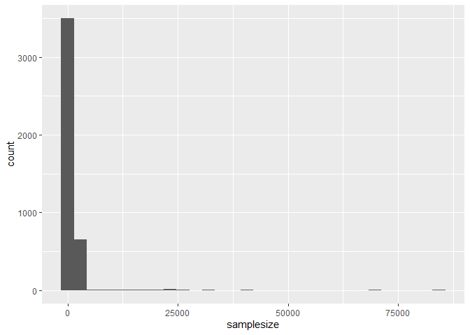
To assess patterns in the data we can visualize the
summaries using histograms and boxplots. Here we will make plots
using the ggplot2 package.
ggplot(data = polls, aes(x = samplesize)) +
  geom_histogram()
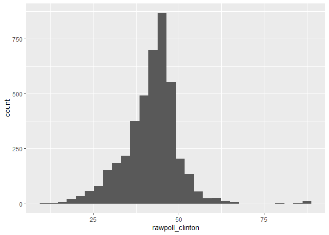
ggplot(data = polls, aes(x = rawpoll_clinton)) +
  geom_histogram()
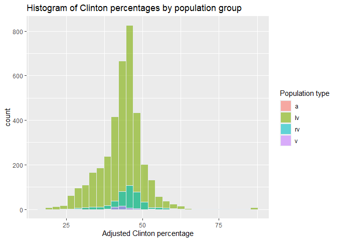
3. Covariance
Looking at histograms by group can tell us whether certain groups tend to be higher or lower and the relative size of different groups. For instance, in this histogram, the group for population type lv has much momre data (higher counts) but the Clinton percentages for this group are not higher or lower than the others.
ggplot(polls, aes(x=adjpoll_clinton, fill=factor(population))) +
  geom_histogram(color="#e9ecef", alpha=0.6, position = 'identity') +
  labs(title = "Histogram of Clinton percentages by population group",
       x = "Adjusted Clinton percentage",
       fill = "Population type")
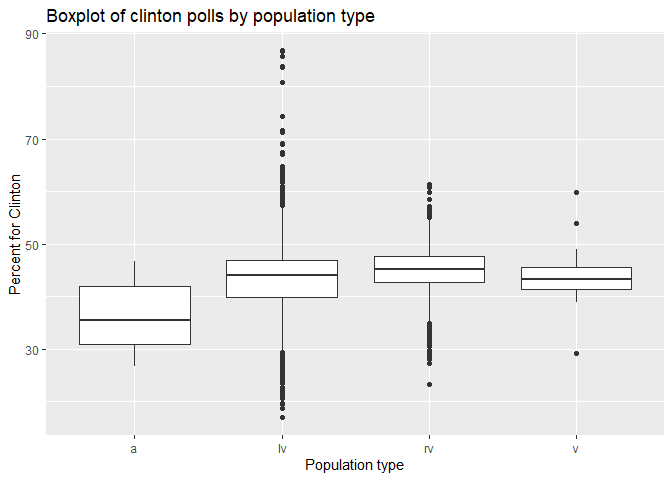
Boxplots can also show the differences …
ggplot(polls, aes(x=factor(population), y=adjpoll_clinton)) +
  geom_boxplot() +
  labs(y = "Percent for Clinton",
       x = "Population type",
       title = "Boxplot of clinton polls by population type")
Correlations show which variables are related. Correlation is only
calculated for numeric variables so we need to select the numeric
variables first. Here we show two ways to calculate the correlation
among variabels. First we use the cor() function from base R.
polls_numeric <- polls %>% dplyr::select(where(is.numeric))

# Base R
corvar = round(cor(polls_numeric, use="complete.obs"), 2)
print(corvar)
##                  samplesize rawpoll_clinton rawpoll_trump rawpoll_johnson
## samplesize             1.00            0.43          0.23           -0.22
## rawpoll_clinton        0.43            1.00          0.03           -0.19
## rawpoll_trump          0.23            0.03          1.00           -0.18
## rawpoll_johnson       -0.22           -0.19         -0.18            1.00
## rawpoll_mcmullin       0.18            0.25         -0.31           -0.71
## adjpoll_clinton        0.21            0.86         -0.13           -0.02
## adjpoll_trump         -0.17           -0.28          0.79            0.13
## adjpoll_johnson       -0.36           -0.33          0.05            0.85
## adjpoll_mcmullin       0.16            0.22         -0.33           -0.69
##                  rawpoll_mcmullin adjpoll_clinton adjpoll_trump adjpoll_johnson
## samplesize                   0.18            0.21         -0.17           -0.36
## rawpoll_clinton              0.25            0.86         -0.28           -0.33
## rawpoll_trump               -0.31           -0.13          0.79            0.05
## rawpoll_johnson             -0.71           -0.02          0.13            0.85
## rawpoll_mcmullin             1.00           -0.02         -0.65           -0.75
## adjpoll_clinton             -0.02            1.00         -0.17           -0.12
## adjpoll_trump               -0.65           -0.17          1.00            0.35
## adjpoll_johnson             -0.75           -0.12          0.35            1.00
## adjpoll_mcmullin             1.00           -0.05         -0.67           -0.75
##                  adjpoll_mcmullin
## samplesize                   0.16
## rawpoll_clinton              0.22
## rawpoll_trump               -0.33
## rawpoll_johnson             -0.69
## rawpoll_mcmullin             1.00
## adjpoll_clinton             -0.05
## adjpoll_trump               -0.67
## adjpoll_johnson             -0.75
## adjpoll_mcmullin             1.00
#Hmisc
library(Hmisc)
rcorr(as.matrix(polls_numeric))
##                  samplesize rawpoll_clinton rawpoll_trump rawpoll_johnson
## samplesize             1.00            0.06         -0.01           -0.01
## rawpoll_clinton        0.06            1.00         -0.44           -0.30
## rawpoll_trump         -0.01           -0.44          1.00           -0.14
## rawpoll_johnson       -0.01           -0.30         -0.14            1.00
## rawpoll_mcmullin       0.18            0.25         -0.31           -0.71
## adjpoll_clinton        0.06            0.92         -0.64           -0.26
## adjpoll_trump         -0.02           -0.66          0.90           -0.04
## adjpoll_johnson       -0.05           -0.26         -0.04            0.84
## adjpoll_mcmullin       0.16            0.22         -0.33           -0.69
##                  rawpoll_mcmullin adjpoll_clinton adjpoll_trump adjpoll_johnson
## samplesize                   0.18            0.06         -0.02           -0.05
## rawpoll_clinton              0.25            0.92         -0.66           -0.26
## rawpoll_trump               -0.31           -0.64          0.90           -0.04
## rawpoll_johnson             -0.71           -0.26         -0.04            0.84
## rawpoll_mcmullin             1.00           -0.02         -0.65           -0.75
## adjpoll_clinton             -0.02            1.00         -0.73           -0.29
## adjpoll_trump               -0.65           -0.73          1.00           -0.05
## adjpoll_johnson             -0.75           -0.29         -0.05            1.00
## adjpoll_mcmullin             1.00           -0.05         -0.67           -0.75
##                  adjpoll_mcmullin
## samplesize                   0.16
## rawpoll_clinton              0.22
## rawpoll_trump               -0.33
## rawpoll_johnson             -0.69
## rawpoll_mcmullin             1.00
## adjpoll_clinton             -0.05
## adjpoll_trump               -0.67
## adjpoll_johnson             -0.75
## adjpoll_mcmullin             1.00
##
## n
##                  samplesize rawpoll_clinton rawpoll_trump rawpoll_johnson
## samplesize             4207            4207          4207            2798
## rawpoll_clinton        4207            4208          4208            2799
## rawpoll_trump          4207            4208          4208            2799
## rawpoll_johnson        2798            2799          2799            2799
## rawpoll_mcmullin         30              30            30              30
## adjpoll_clinton        4207            4208          4208            2799
## adjpoll_trump          4207            4208          4208            2799
## adjpoll_johnson        2798            2799          2799            2799
## adjpoll_mcmullin         30              30            30              30
##                  rawpoll_mcmullin adjpoll_clinton adjpoll_trump adjpoll_johnson
## samplesize                     30            4207          4207            2798
## rawpoll_clinton                30            4208          4208            2799
## rawpoll_trump                  30            4208          4208            2799
## rawpoll_johnson                30            2799          2799            2799
## rawpoll_mcmullin               30              30            30              30
## adjpoll_clinton                30            4208          4208            2799
## adjpoll_trump                  30            4208          4208            2799
## adjpoll_johnson                30            2799          2799            2799
## adjpoll_mcmullin               30              30            30              30
##                  adjpoll_mcmullin
## samplesize                     30
## rawpoll_clinton                30
## rawpoll_trump                  30
## rawpoll_johnson                30
## rawpoll_mcmullin               30
## adjpoll_clinton                30
## adjpoll_trump                  30
## adjpoll_johnson                30
## adjpoll_mcmullin               30
##
## P
##                  samplesize rawpoll_clinton rawpoll_trump rawpoll_johnson
## samplesize                  0.0000          0.5954        0.4689
## rawpoll_clinton  0.0000                     0.0000        0.0000
## rawpoll_trump    0.5954     0.0000                        0.0000
## rawpoll_johnson  0.4689     0.0000          0.0000
## rawpoll_mcmullin 0.3356     0.1888          0.0984        0.0000
## adjpoll_clinton  0.0002     0.0000          0.0000        0.0000
## adjpoll_trump    0.1590     0.0000          0.0000        0.0339
## adjpoll_johnson  0.0053     0.0000          0.0275        0.0000
## adjpoll_mcmullin 0.3984     0.2434          0.0706        0.0000
##                  rawpoll_mcmullin adjpoll_clinton adjpoll_trump adjpoll_johnson
## samplesize       0.3356           0.0002          0.1590        0.0053
## rawpoll_clinton  0.1888           0.0000          0.0000        0.0000
## rawpoll_trump    0.0984           0.0000          0.0000        0.0275
## rawpoll_johnson  0.0000           0.0000          0.0339        0.0000
## rawpoll_mcmullin                  0.9226          0.0000        0.0000
## adjpoll_clinton  0.9226                           0.0000        0.0000
## adjpoll_trump    0.0000           0.0000                        0.0088
## adjpoll_johnson  0.0000           0.0000          0.0088
## adjpoll_mcmullin 0.0000           0.8085          0.0000        0.0000
##                  adjpoll_mcmullin
## samplesize       0.3984
## rawpoll_clinton  0.2434
## rawpoll_trump    0.0706
## rawpoll_johnson  0.0000
## rawpoll_mcmullin 0.0000
## adjpoll_clinton  0.8085
## adjpoll_trump    0.0000
## adjpoll_johnson  0.0000
## adjpoll_mcmullin
#Corrplot
library(corrplot)
corrplot(corvar, type = "upper", order = "hclust",
         tl.col = "black", tl.srt = 45)
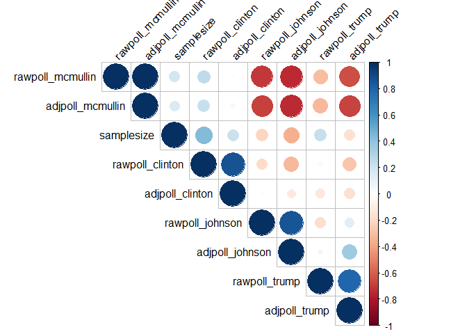
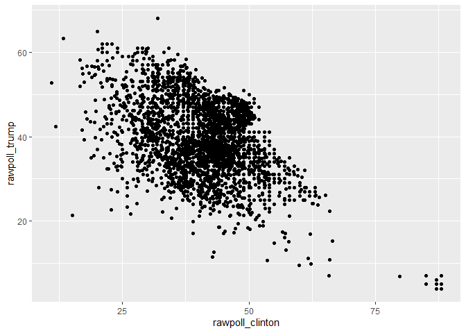
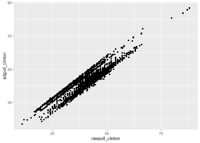
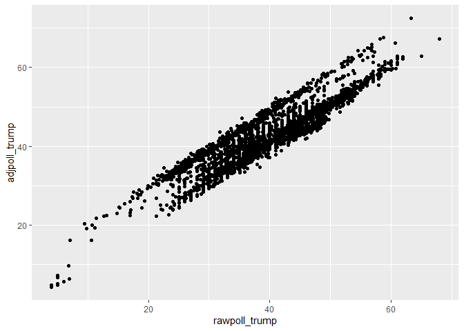
Scatter plots are useful to look at bivariate relationships: how two variables are related to each other.
ggplot(polls, aes(x=rawpoll_clinton, y=rawpoll_trump)) + geom_point()
ggplot(polls, aes(x=rawpoll_clinton, y=adjpoll_clinton)) + geom_point()
ggplot(polls, aes(x=rawpoll_trump, y=adjpoll_trump)) + geom_point()
Helpful packages
For this section we will use a variety of packages. To make sure that
these packages are installed run the install.packages() command
introduced above (if you have not already done so).
skimr:
Sometimes you need a quick look at the data and want to view many of the
EDA summaries and visualizations together. The skimr package automates
summaries for variables by giving an overview of the data, then
summarizing character, Date, factor, and numeric data.
library(skimr)
skim(polls)
| | | | :———————————————– | :—- | | Name | polls | | Number of rows | 4208 | | Number of columns | 15 | | _______________________ | | | Column type frequency: | | | character | 1 | | Date | 2 | | factor | 3 | | numeric | 9 | | ________________________ | | | Group variables | None |
Data summary
Variable type: character
| skim_variable | n_missing | complete_rate | min | max | empty | n_unique | whitespace |
|---|---|---|---|---|---|---|---|
| population | 0 | 1 | 1 | 2 | 0 | 4 | 0 |
Variable type: Date
| skim_variable | n_missing | complete_rate | min | max | median | n_unique |
|---|---|---|---|---|---|---|
| startdate | 0 | 1 | 2015-11-06 | 2016-11-06 | 2016-09-23 | 352 |
| enddate | 0 | 1 | 2015-11-08 | 2016-11-07 | 2016-09-30 | 345 |
Variable type: factor
| skim_variable | n_missing | complete_rate | ordered | n_unique | top_counts |
|---|---|---|---|---|---|
| state | 0 | 1.0 | FALSE | 57 | U.S: 1106, Flo: 148, Nor: 125, Pen: 125 |
| pollster | 0 | 1.0 | FALSE | 196 | Ips: 919, Goo: 743, Sur: 660, You: 130 |
| grade | 429 | 0.9 | FALSE | 10 | A-: 1085, B: 1011, C-: 693, C+: 329 |
Variable type: numeric
| skim_variable | n_missing | complete_rate | mean | sd | p0 | p25 | p50 | p75 | p100 | hist |
|---|---|---|---|---|---|---|---|---|---|---|
| samplesize | 1 | 1.00 | 1148.22 | 2630.86 | 35.00 | 447.50 | 772.00 | 1236.50 | 84292.00 | ▇▁▁▁▁ |
| rawpoll_clinton | 0 | 1.00 | 41.99 | 7.73 | 11.04 | 38.00 | 43.00 | 46.20 | 88.00 | ▁▅▇▁▁ |
| rawpoll_trump | 0 | 1.00 | 39.83 | 7.88 | 4.00 | 35.00 | 40.00 | 45.00 | 68.00 | ▁▁▇▅▁ |
| rawpoll_johnson | 1409 | 0.67 | 7.38 | 2.96 | 0.00 | 5.40 | 7.00 | 9.00 | 25.00 | ▃▇▂▁▁ |
| rawpoll_mcmullin | 4178 | 0.01 | 24.00 | 5.70 | 9.00 | 22.50 | 25.00 | 27.90 | 31.00 | ▂▁▃▇▇ |
| adjpoll_clinton | 0 | 1.00 | 43.32 | 7.09 | 17.06 | 40.21 | 44.15 | 46.92 | 86.77 | ▁▇▆▁▁ |
| adjpoll_trump | 0 | 1.00 | 42.67 | 6.95 | 4.37 | 38.43 | 42.76 | 46.29 | 72.43 | ▁▁▇▃▁ |
| adjpoll_johnson | 1409 | 0.67 | 4.66 | 2.47 | -3.67 | 3.15 | 4.38 | 5.76 | 20.37 | ▁▇▂▁▁ |
| adjpoll_mcmullin | 4178 | 0.01 | 24.51 | 5.24 | 11.03 | 23.11 | 25.14 | 27.98 | 31.57 | ▂▁▂▇▆ |
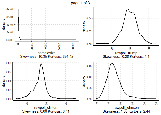
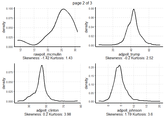
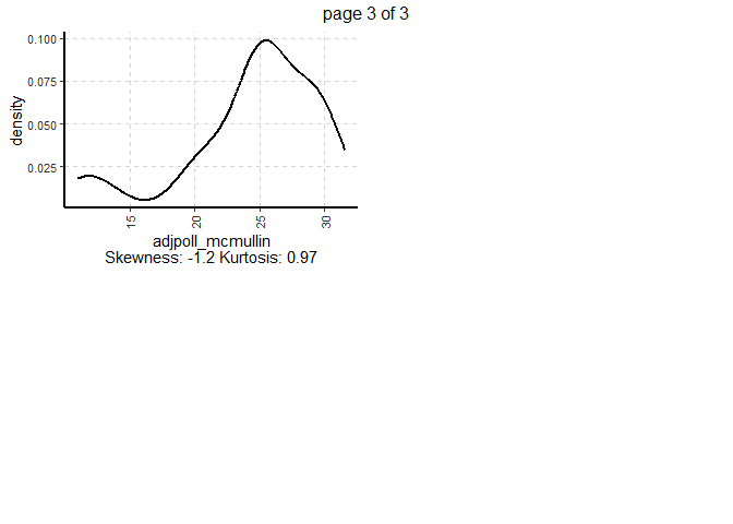
smartEDA:
The SmartEDA package has an impressive range of capabilities. It
provides variable summaries, density plots, the distribution of
categorical variables, scatter plots of each variable against a target
variable, calculation of chi-squared and p-values for each variable as a
predictor of a target variable, Q-Q plots for continuous variables,
parallel coordinate plots, and more. This
vignette
gives a full demonstration of the power of SmartEDA. Here are a few
small examples of what it can do.
library(SmartEDA)
ExpData(data = polls, type = 2)
##    Index    Variable_Name Variable_Type Per_of_Missing No_of_distinct_values
## 1      1            state        factor        0.00000                    57
## 2      2        startdate          Date        0.00000                   352
## 3      3          enddate          Date        0.00000                   345
## 4      4         pollster        factor        0.00000                   196
## 5      5            grade        factor        0.10195                    11
## 6      6       samplesize       integer        0.00024                  1767
## 7      7       population     character        0.00000                     4
## 8      8  rawpoll_clinton       numeric        0.00000                  1312
## 9      9    rawpoll_trump       numeric        0.00000                  1385
## 10    10  rawpoll_johnson       numeric        0.33484                   585
## 11    11 rawpoll_mcmullin       numeric        0.99287                    17
## 12    12  adjpoll_clinton       numeric        0.00000                  4200
## 13    13    adjpoll_trump       numeric        0.00000                  4204
## 14    14  adjpoll_johnson       numeric        0.33484                  2211
## 15    15 adjpoll_mcmullin       numeric        0.99287                    31
ExpNumViz(polls,
          target = NULL,
          nlim = 10,
          Page = c(2,2))[[1]]
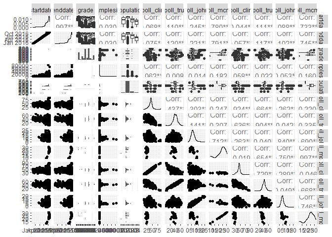
GGally:
The ggpairs() function from the GGally package creates plots of each
variable against all others. For categorical variables ggpairs is
limited to 15 categories. The variables state and pollster have
momre than 15 unique values so we removed them from the polls data
before plotting.
library('GGally')
ggpairs(polls[,-c(1,4)])
Hmisc:
library(Hmisc)
Hmisc::describe(polls)
## polls
##
##  15  Variables      4208  Observations
## --------------------------------------------------------------------------------
## state
##        n  missing distinct
##     4208        0       57
##
## lowest : Alabama       Alaska        Arizona       Arkansas      California
## highest: Virginia      Washington    West Virginia Wisconsin     Wyoming
## --------------------------------------------------------------------------------
## startdate
##          n    missing   distinct       Info       Mean        Gmd        .05
##       4208          0        352          1 2016-08-31      70.27 2016-03-14
##        .10        .25        .50        .75        .90        .95
## 2016-05-23 2016-08-10 2016-09-23 2016-10-20 2016-10-29 2016-11-01
##
## lowest : 2015-11-06 2015-11-07 2015-11-09 2015-11-10 2015-11-11
## highest: 2016-11-02 2016-11-03 2016-11-04 2016-11-05 2016-11-06
## --------------------------------------------------------------------------------
## enddate
##          n    missing   distinct       Info       Mean        Gmd        .05
##       4208          0        345          1 2016-09-06      70.47 2016-03-18
##        .10        .25        .50        .75        .90        .95
## 2016-05-26 2016-08-21 2016-09-30 2016-10-28 2016-11-03 2016-11-06
##
## lowest : 2015-11-08 2015-11-13 2015-11-15 2015-11-16 2015-11-17
## highest: 2016-11-03 2016-11-04 2016-11-05 2016-11-06 2016-11-07
## --------------------------------------------------------------------------------
## pollster
##        n  missing distinct
##     4208        0      196
##
## lowest : ABC News/Washington Post       American Research Group        American Strategies            Angus Reid Global              Anzalone Liszt Grove Research
## highest: Winthrop University            Y2 Analytics                   YouGov                         Zia Poll                       Zogby Interactive/JZ Analytics
## --------------------------------------------------------------------------------
## grade
##        n  missing distinct
##     3779      429       10
##
## lowest : D  C- C  C+ B-, highest: B  B+ A- A  A+
##
## Value          D    C-     C    C+    B-     B    B+    A-     A    A+
## Frequency     14   693    58   329   142  1011   204  1085   159    84
## Proportion 0.004 0.183 0.015 0.087 0.038 0.268 0.054 0.287 0.042 0.022
## --------------------------------------------------------------------------------
## samplesize
##        n  missing distinct     Info     Mean      Gmd      .05      .10
##     4207        1     1766        1     1148     1142    137.0    244.0
##      .25      .50      .75      .90      .95
##    447.5    772.0   1236.5   1951.8   2562.4
##
## lowest :    35    37    39    42    43, highest: 32225 32226 40816 70194 84292
## --------------------------------------------------------------------------------
## population
##        n  missing distinct
##     4208        0        4
##
## Value          a    lv    rv     v
## Frequency     21  3727   418    42
## Proportion 0.005 0.886 0.099 0.010
## --------------------------------------------------------------------------------
## rawpoll_clinton
##        n  missing distinct     Info     Mean      Gmd      .05      .10
##     4208        0     1312        1    41.99    8.237    28.08    31.50
##      .25      .50      .75      .90      .95
##    38.00    43.00    46.20    49.94    52.71
##
## lowest : 11.04 11.78 13.34 15.11 16.57, highest: 66.53 79.80 85.00 87.00 88.00
## --------------------------------------------------------------------------------
## rawpoll_trump
##        n  missing distinct     Info     Mean      Gmd      .05      .10
##     4208        0     1385        1    39.83    8.722    27.00    30.00
##      .25      .50      .75      .90      .95
##    35.00    40.00    45.00    49.09    53.00
##
## lowest :  4.00  5.00  6.00  6.80  7.00, highest: 61.00 62.00 63.29 65.00 68.00
## --------------------------------------------------------------------------------
## rawpoll_johnson
##        n  missing distinct     Info     Mean      Gmd      .05      .10
##     2799     1409      584    0.997    7.382     3.19     3.00     4.00
##      .25      .50      .75      .90      .95
##     5.40     7.00     9.00    11.00    12.95
##
## lowest :  0.00  0.98  1.00  1.32  1.49, highest: 21.00 22.00 23.00 24.00 25.00
## --------------------------------------------------------------------------------
## rawpoll_mcmullin
##        n  missing distinct     Info     Mean      Gmd      .05      .10
##       30     4178       16     0.99       24    5.943    10.35    17.40
##      .25      .50      .75      .90      .95
##    22.50    25.00    27.90    29.00    29.55
##
## lowest :  9.0 12.0 18.0 20.0 21.0, highest: 27.6 28.0 29.0 30.0 31.0
##
## Value       9.00 12.00 18.00 20.00 21.00 22.00 24.00 24.52 25.00 26.00 27.00
## Frequency      2     1     1     2     1     1     3     1     4     4     1
## Proportion 0.067 0.033 0.033 0.067 0.033 0.033 0.100 0.033 0.133 0.133 0.033
##
## Value      27.60 28.00 29.00 30.00 31.00
## Frequency      1     1     5     1     1
## Proportion 0.033 0.033 0.167 0.033 0.033
## --------------------------------------------------------------------------------
## adjpoll_clinton
##        n  missing distinct     Info     Mean      Gmd      .05      .10
##     4208        0     4200        1    43.32    7.465    30.03    33.62
##      .25      .50      .75      .90      .95
##    40.21    44.15    46.92    50.43    53.38
##
## lowest : 17.06495 18.62685 19.41599 19.60153 19.61379
## highest: 85.77880 86.64585 86.70544 86.76118 86.77218
## --------------------------------------------------------------------------------
## adjpoll_trump
##        n  missing distinct     Info     Mean      Gmd      .05      .10
##     4208        0     4204        1    42.67    7.524    32.12    34.68
##      .25      .50      .75      .90      .95
##    38.43    42.76    46.29    51.33    54.35
##
## lowest :  4.372936  4.622556  4.862200  4.879020  5.103538
## highest: 66.183890 67.167230 67.314490 67.607800 72.433030
## --------------------------------------------------------------------------------
## adjpoll_johnson
##        n  missing distinct     Info     Mean      Gmd      .05      .10
##     2799     1409     2210        1     4.66    2.612    1.283    1.996
##      .25      .50      .75      .90      .95
##    3.145    4.384    5.756    7.648    8.988
##
## lowest : -3.667890 -3.011773 -2.928394 -1.361062 -1.168077
## highest: 16.342580 17.234500 17.988220 19.364130 20.366840
## --------------------------------------------------------------------------------
## adjpoll_mcmullin
##        n  missing distinct     Info     Mean      Gmd      .05      .10
##       30     4178       30        1    24.51    5.613    12.51    18.36
##      .25      .50      .75      .90      .95
##    23.11    25.14    27.98    29.65    30.06
##
## lowest : 11.02832 11.56920 13.65646 18.87894 20.74372
## highest: 29.47327 29.64230 29.67611 30.37186 31.57469
## --------------------------------------------------------------------------------
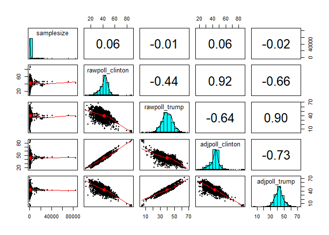
Psych:
library(psych)
psych::describe(polls)
##                  vars    n    mean      sd median trimmed    mad   min      max
## state*              1 4208   34.47   17.03  39.00   35.84  16.31  1.00    57.00
## startdate           2 4208     NaN      NA     NA     NaN     NA   Inf     -Inf
## enddate             3 4208     NaN      NA     NA     NaN     NA   Inf     -Inf
## pollster*           4 4208  104.10   48.61  81.00  103.27  41.51  1.00   196.00
## grade*              5 3779    5.83    2.34   6.00    5.94   2.97  1.00    10.00
## samplesize          6 4207 1148.22 2630.86 772.00  837.95 548.56 35.00 84292.00
## population*         7 4208    2.11    0.36   2.00    2.01   0.00  1.00     4.00
## rawpoll_clinton     8 4208   41.99    7.73  43.00   42.29   5.93 11.04    88.00
## rawpoll_trump       9 4208   39.83    7.88  40.00   39.92   7.41  4.00    68.00
## rawpoll_johnson    10 2799    7.38    2.96   7.00    7.16   2.97  0.00    25.00
## rawpoll_mcmullin   11   30   24.00    5.70  25.00   25.00   4.45  9.00    31.00
## adjpoll_clinton    12 4208   43.32    7.09  44.15   43.55   4.79 17.06    86.77
## adjpoll_trump      13 4208   42.67    6.95  42.76   42.60   5.73  4.37    72.43
## adjpoll_johnson    14 2799    4.66    2.47   4.38    4.47   1.91 -3.67    20.37
## adjpoll_mcmullin   15   30   24.51    5.24  25.14   25.31   4.08 11.03    31.57
##                     range  skew kurtosis    se
## state*              56.00 -0.54    -1.18  0.26
## startdate            -Inf    NA       NA    NA
## enddate              -Inf    NA       NA    NA
## pollster*          195.00  0.24    -1.12  0.75
## grade*               9.00 -0.45    -0.96  0.04
## samplesize       84257.00 16.34   391.23 40.56
## population*          3.00  2.69     8.34  0.01
## rawpoll_clinton     76.96  0.06     3.41  0.12
## rawpoll_trump       64.00 -0.28     1.10  0.12
## rawpoll_johnson     25.00  1.03     2.43  0.06
## rawpoll_mcmullin    22.00 -1.35     1.14  1.04
## adjpoll_clinton     69.71  0.20     3.98  0.11
## adjpoll_trump       68.06 -0.20     2.52  0.11
## adjpoll_johnson     24.03  1.19     3.59  0.05
## adjpoll_mcmullin    20.55 -1.14     0.71  0.96
pairs.panels(polls[,c(6,8,9,12,13)])
summarytools:
The summarytools package gives descriptive statistics for the
continuous variables using descr(). You can also get the frequency of
each category for factors using the dfSummary() function.
library(summarytools)
summarytools::descr(polls)
## Descriptive Statistics
## polls
## N: 4208
##
##                     adjpoll_clinton   adjpoll_johnson   adjpoll_mcmullin   adjpoll_trump
## ----------------- ----------------- ----------------- ------------------ ---------------
##              Mean             43.32              4.66              24.51           42.67
##           Std.Dev              7.09              2.47               5.24            6.95
##               Min             17.06             -3.67              11.03            4.37
##                Q1             40.21              3.15              22.81           38.43
##            Median             44.15              4.38              25.14           42.76
##                Q3             46.92              5.76              28.07           46.29
##               Max             86.77             20.37              31.57           72.43
##               MAD              4.79              1.91               4.08            5.73
##               IQR              6.71              2.61               4.87            7.86
##                CV              0.16              0.53               0.21            0.16
##          Skewness              0.20              1.19              -1.14           -0.20
##       SE.Skewness              0.04              0.05               0.43            0.04
##          Kurtosis              3.98              3.59               0.71            2.52
##           N.Valid           4208.00           2799.00              30.00         4208.00
##         Pct.Valid            100.00             66.52               0.71          100.00
##
## Table: Table continues below
##
##
##
##                     rawpoll_clinton   rawpoll_johnson   rawpoll_mcmullin   rawpoll_trump   samplesize
## ----------------- ----------------- ----------------- ------------------ --------------- ------------
##              Mean             41.99              7.38              24.00           39.83      1148.22
##           Std.Dev              7.73              2.96               5.70            7.88      2630.86
##               Min             11.04              0.00               9.00            4.00        35.00
##                Q1             38.00              5.40              22.00           35.00       447.00
##            Median             43.00              7.00              25.00           40.00       772.00
##                Q3             46.20              9.00              28.00           45.00      1237.00
##               Max             88.00             25.00              31.00           68.00     84292.00
##               MAD              5.93              2.97               4.45            7.41       548.56
##               IQR              8.20              3.60               5.40           10.00       789.00
##                CV              0.18              0.40               0.24            0.20         2.29
##          Skewness              0.06              1.03              -1.35           -0.28        16.34
##       SE.Skewness              0.04              0.05               0.43            0.04         0.04
##          Kurtosis              3.41              2.43               1.14            1.10       391.23
##           N.Valid           4208.00           2799.00              30.00         4208.00      4207.00
##         Pct.Valid            100.00             66.52               0.71          100.00        99.98
summarytools::dfSummary(polls$grade)
## Data Frame Summary
## polls
## Dimensions: 4208 x 1
## Duplicates: 4197
##
## --------------------------------------------------------------------------------------
## No   Variable   Stats / Values   Freqs (% of Valid)   Graph      Valid      Missing
## ---- ---------- ---------------- -------------------- ---------- ---------- ----------
## 1    grade      1. D               14 ( 0.4%)                    3779       429
##      [factor]   2. C-             693 (18.3%)         III        (89.81%)   (10.19%)
##                 3. C               58 ( 1.5%)
##                 4. C+             329 ( 8.7%)         I
##                 5. B-             142 ( 3.8%)
##                 6. B             1011 (26.8%)         IIIII
##                 7. B+             204 ( 5.4%)         I
##                 8. A-            1085 (28.7%)         IIIII
##                 9. A              159 ( 4.2%)
##                 10. A+             84 ( 2.2%)
## --------------------------------------------------------------------------------------
Two other packages to check out are RtutoR and DataExplorer see
this article.
Conclusion
EDA can be insightful and is a necessary first step!