
An R Case Study - The effect of nutrient loading on canopy diversity
This project started as a class project but it is a good showcase of a Bayesian mixed model in R.
Research Questions
- To what extent does a low nitrogen impacted forest in the US exhibit loss of biodiversity with increased soil nitrogen? (Are these “natural” forests already in a state of nutrient excess?)
- What drives the percent basal area (BA) of the dominant canopy species (with respect to the relative importance of climate, soil nutrients, and species-specific characteristics)?
Overview
Though nutrient increases are typically viewed as a benefit for ecosystems, increasing productivity and diversity, excess nutrients – especially nitrogen – can depress diversity eliciting cascades of effects fundamentally changing ecosystem structure. With the continued rise of nitrogen based fertilizers and increasing rates of nitrogen deposition stemming from air pollution, ecosystem management requires a deeper understanding of the impacts that excess nutrients will have on ecosystem diversity. Through a statistical model of a low impact ecosystem in the Pacific Northwest of the United States, latitude, soil nitrogen, soil pH and mean annual temperature were shown to be the strongest drivers of forest diversity in a relatively natural condition forest. As soil nitrogen levels increased, diversity increased demonstrating that low impacted forests behave in a profoundly different way from disturbed ecosystems that decrease diversity with rising nitrogen levels. The model also demonstrated the difference in response trajectories among different genera of plants supporting the theory that ecosystems of different compositions will respond differently to enhanced nutrient loading.
Data set
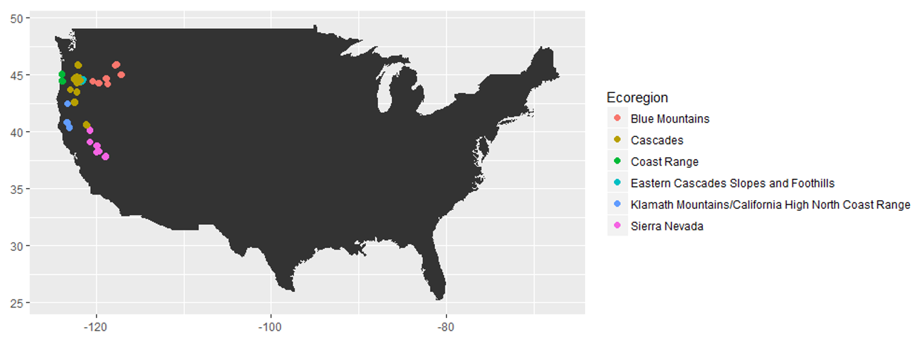
The NACP Terrestrial Ecosystem Research and Regional Analysis – Pacific Northwest (TERRA-PNW) data set was used for this analysis. The data set contains forest plant traits, biomass, and soil properties analysis from 1999 through 2004 in Oregon and Northern California. A total of 212 1-hectare plots were analyzed for this paper. The forested areas in the Pacific Northwest can be divided into six ecoregions based on geographic and climatic differences: Blue Mountains, Coastal Range, Eastern Cascades, Klamath Mountains, Sierra Nevada Mountains, and the Western Cascades. Within each ecoregion the species composition and climate are comparable making this a possible grouping factor that accounts for some effects of climate and species-specific effects.
Model
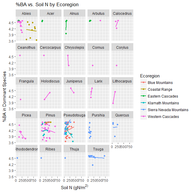
Initial data exploration demonstrated a relationship between soil nitrogen and percent BA when plots were broken down by dominant species genus and ecoregion. Figure 1 shows that different genera display different dominance responses to changing soil nitrogen and that the relationship depends on the ecoregion of plot. This indicates that both climatic factors (encompassed in the different ecoregions) and different plant physiologies (encompassed in the different genera) impacted a stand’s response to changing nitrogen levels. These characteristics were included during variable selection.
Variable selection was conducted to reduce the number of covariates (therefore minimizing the degrees of freedom and maximizing the model’s power) based on autocorrelation among variables, coefficient effects in generalized linear models, and biological justification. Correlation among covariates is shown here:
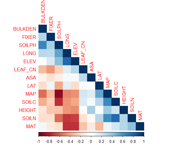
Soil pH was highly correlated with both mean annual precipitation and soil carbon resulting in the removal of precipitation and carbon from the model. pH has important effects on nutrient solubility and therefore availability to plants rendering it a critical factor to incorporate into the model. Longitude was highly correlated with soil nitrogen and mean annual temperature so it was removed from the model. After removing covariates with high correlation, general linear models were developed to test coefficient effect of the remaining covariates as shown here:
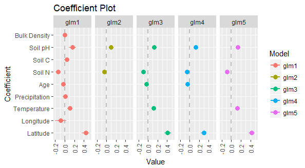
In the coefficient plot, factors whose 95% credible interval does not cross the 0 line are significant. The four most significant variables were: latitude, mean annual temperature, soil nitrogen, and soil pH. Models were further tested dropping one covariate at a time to evaluate the impact of removing any one of these covariates. The results of the drop one test are shown in Table 2 and indicate that, although the strength of impact varies, all four factors are important to the overall model. These factors were carried forward into the mixed model development.

Mixed models were subsequently developed with the covariates selected through variable selection included as fixed effects and random effects applied through grouping factors. The models were optimized using restricted maximum likelihood because the structure of the fixed effects did not vary among the models rather the random effects (grouping factors) were manipulated. Grouping factors considered were: plot number, ecoregion, and genus. Due to low counts in many species, plants were aggregated at the genus level to reduce effects of small sample sizes. Models with plot number and ecoregion performed poorly compared with those incorporating genus as a random effect. Though when combined, genus and ecoregion together produced a good fit. Ultimately the three models performing highest in terms of AIC, DIC, deviance were those using genus as a random effect (either as intercept, slope and intercept, or intercept along with ecoregion). Model selection is described further in the model evaluation section.
Bayesian Framework
These models were developed in a Bayesian framework indicating that the posterior, likelihood, and prior were all distributions which facilitated a full incorporation of uncertainty into the model. Using a Bayesian framework also incorporates prior information which can increase the value of the posterior distribution. Bayesian frameworks consider parameters as random variables that update prior knowledge. The marginal distribution was computed using a Markov chain Monte Carlo (MCMC) algorithm with 50,000 iterations and 1,000 iterations removed as burn-in. The MCMC algorithm used a Metropolis-Hastings update criterion. Uninformative priors were used as there was not existing data relevant to incorporate as prior information. With a fairly large sample size (212 plots), the likelihood distribution dominates over the priors weighting the new information more heavily than the uninformative prior starting position. The posterior distribution can be written as:

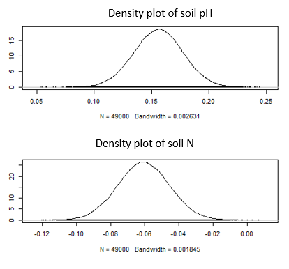
This indicates that the probability of the parameters given the data is proportional to the probability of the data given the parameters times the prior distributions of the parameters. In these models there are four parameters for the coefficient of each covariate. The posterior distribution is found using the MCMC algorithm and an example distribution for soil nitrogen and soil pH are shown here:
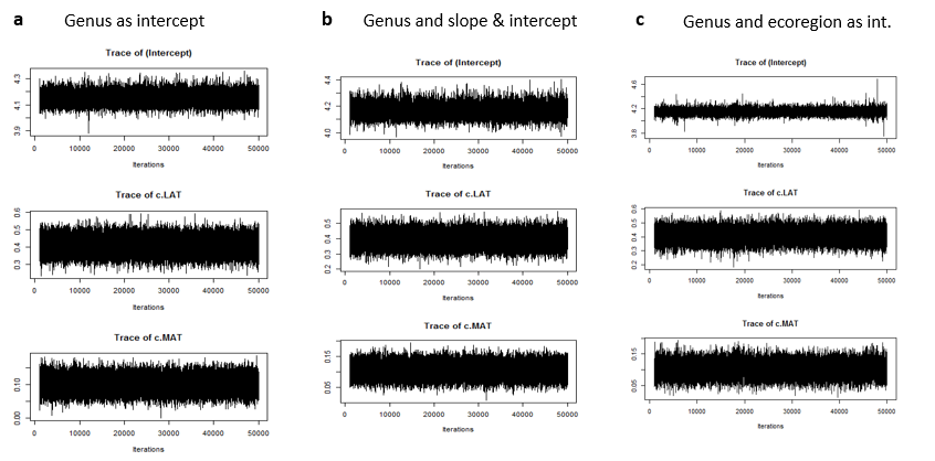
The mixed effect models (with both fixed and random effects) were incorporated into the Bayesian framework. The trace plots below were used for visual inspection of model convergence. All trace plots demonstrate good convergence in the MCMC chains for each parameter and show the posterior distributions for each parameter. The parameters shown in were z-transformed for standardization.
Model Evaluation
Various models were developed using the covariates found during variable selection and a range of random effects. The random effects including grouping factors of plot number, genus, and ecoregion applied as slope, intercept, or both in different combinations. Based on Figure 1 both genus and ecoregion has an impact on the shape of the relationship between soil nitrogen and diversity. The three top performing models (which performed similarly under several model selection criteria) are presented here. Deviance is a measure of model fit which is useful for model evaluation. The lower the deviance, the better the fit between the model and data. However, complexity must also be considered since a good fit with too much complexity is meaningless (Spiegelhalter, 2002). Tradeoffs between these two capacities is quantified using the Akaike Information Criterion (AIC). AIC values are presented here for model comparison.
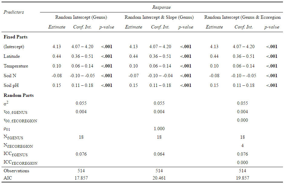
The table shows the intraclass correlation coefficient (ICC) for each of the models based on grouping factors. The ICC is a metric that measures the ratio of variance within the class compared to total variance. When ecoregion is used as a grouping factor the ICC is zero which indicates there is no statistical need to use this grouping factor. However, there is biological justification for including the ecoregion as a random effect since plant diversity is closely linked to climate variables which change across ecoregions. The AIC values are also shown in Table 3 with lower AIC generally indicating a better model in terms of fit penalized for parameters. The first model (genus as intercept) has the lowest AIC at 17.857, however, an AIC of 4-6 is generally required to demonstrate a meaningful difference between models and difference of 10 to be sure the models are different. Here the models perform similarly based on AIC and so are all included as the best models.
Model assumptions were also tested including the normality of variance, homogeneity of variance, and independence of data. Linear mixed effects models assume that residuals are normally distributed. This was verified by visual inspection of the Q-Q plot shown here:
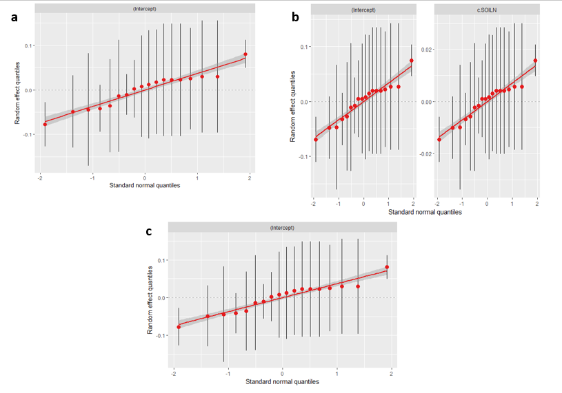
Residuals adhering to this assumption fall directly on the Q-Q line which is demonstrated in the figure. Furthermore, linear mixed effect models assume that the variance is distributed approximately homogeneously among groups. This was verified by visual examination of Pearson fitted values versus residuals. The variances were approximately homogenous indicating that the linear mixed effect model can be appropriately applied to this data.
The fit between predicted data and observed data was examined using both conditional R2 and marginal R2. Conditional R2 describes the variance from both random and fixed effects while the marginal R2 describes the variance explained by fixed effects alone.

While the conditional R2 values are greater than the marginal R2s for each of the models, the majority of the variance is explained by the fixed effects indicating that the grouping factors had a relatively limited impact on the relationship between soil nitrogen and diversity. Instead, the fixed effects (latitude, temperature, soil nitrogen, and soil pH) are dominating the model. The three models are comparable in terms of R2 further supporting the argument that model selection is not appropriate among these three candidate models.
Results
All three models selected under model evaluation demonstrate similar relationships between covariates and percent BA. Latitude has a strong positive effect on percent BA, temperature and soil pH have a moderate positive effect on percent BA, and soil nitrogen has a negative effect on percent BA. These trends are visualized here:

This indicates that as latitude, temperature, and soil pH increase, the percent BA in the dominant species also increases indicating a decrease in diversity. The trends in latitude and temperature align with results of previous studies indicating that diversity is lower at high latitudes and cold temperatures (Rohde, 1992). The coefficient plots here indicate the strength of effects from different covariates in each of the three best models.
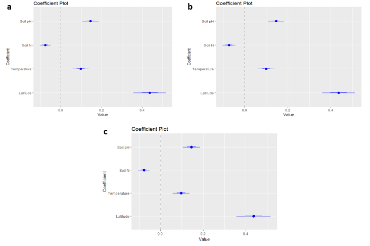
All four covariates are significant coefficients (the 95% confidence interval shown in the thin line does not cross zero). Latitude has the strongest coefficient effect size indicating that it was the primary driver of the pattern in percent BA dominance. The differences among the models are slight and no visible difference is seen among the three coefficient plots. However, the magnitude of the coefficient is not an indication of the coefficient effect. The final model equations are shown in equations 5, 6, and 7 where the largest magnitude coefficient is nitrogen, although the coefficient plots clearly shows that latitude is the most significant driver of percent BA.

In the figure below panel c, the intercept is assigned based on ecoregion. The green line shows the Eastern Cascades region with the greatest intercept indicating that for a given level of soil nitrogen the corresponding percent BA is the largest (or least diverse). This could correspond to the high level of Alnus or Alder trees in those plots which are typically drier plots with larger temperature fluctuations in the rain shadow of the Cascade Mountains. The abundance of shrubs is much greater than trees which might result in Alnus forming a larger percentage of tree/shrub basal area measured. The lowest ecoregion intercept corresponds to the Klamath Mountains, an ecoregion spanning a relatively long latitudinal gradient that encompasses both temperate rainforest and coniferous forest. These gradients align with the observation that the percent BA is generally lower than other ecoregions (therefore the diversity is higher).

In terms of slopes and intercepts observed in panels a and b, the genus corresponding the largest percent BA (lowest diversity) was Pseudotsuga while the other extreme (highest diversity) was characterized by Tsuga. Both of these genera had large sample sizes and therefore the effects are likely representative of forest processes. Pseudotsuga is in the Pinacea family and includes species such as the Douglas Fir and Oregon Pine. This is a fast growing genus and was generally found in younger plots. It is likely that the fast growing Pseudotsuga dominated the stands in these plots due to their fast growth and reduced the diversity. Tsuga is also in the Pinacea family and includes Hemlock trees. These trees require high rainfall and relatively cool temperatures. Due to these physiological constraints, Tsuga primarily appeared in plots with lower mean annual temperature which was highly correlated with high diversity (see Figure 6). The trend in slope by genus mirrored that of the intercepts with Pseudotsuga increasing percent BA fastest as soil nitrogen increased and Tsuga decreasing percent BA as soil nitrogen increased. Additionally, Tsuga was the dominant species in most of the oldest plots (550 years and above). Species diversity tends to increase with forest age until a maximum is achieved and subsequently diversity declines. It is likely that the older plots that include Tsuga.
Discussion
Species diversity within forests is the result of several factors acting in concert. As the soil nitrogen in the plots increased, the diversity in the plots increased (seen as an increased in the percent BA by the dominant species). This trend is opposite to the pattern expected for this region and shown in previous studies such as the grasslands fertilization experiment. This is likely because the forest region analyzed is relatively “natural” with low anthropogenic nitrogen inputs. The ecosystem is limited in nitrogen and therefore areas with additional nitrogen demonstrate more diverse growth. As shown in the results section, latitude and soil pH were the most significant drivers of percent BA in the dominant species. Continuing use of nitrogen-based fertilizer and emission of nitrogen pollutants will continue to raise the level of excess soil nitrogen which depresses diversity within plots. Although other covariates were shown to be more important than soil nitrogen, soil nitrogen had a significant effect which will in turn have significant effects on forest diversity.
The relative effects of coefficients compared to grouping factors is shown by comparing the variance explained by each part of the model. Table 4 shows the relative percentages explained by each part of the model. Since the fixed effects dominated the results, it can be concluded that the fixed effects were are more important driver of diversity trends. In particular, latitude was the primary driver of diversity explaining roughly 55% of the variance accounted for in random effects. Temperature explained around 7% of the variance, soil nitrogen around 10%, and soil pH explained 30% of the variance. This indicates that climate factors had a much stronger impact on diversity trends than soil nutrients. Within the soil properties, pH dominate the impacts over soil nitrogen. Although soil nitrogen was not a top contributor to diversity trends in this data set, it was still a significant covariate and therefore important to consider in forest management. Although wide scale trends may not be driven by soil nutrients, changes in these nutrient levels will still have perceptible ecosystem impacts.
Several of the covariates explored during variable selection did not result in significant trends. Most surprising was that stand age did not affect the percent BA in the dominant species. One possible explanation for this is that the increased mineralization in the older soils was encapsulated by the soil nitrogen measurement and the additional nitrogen available to plants was accounted for through those measurements.